In this challenge, we’re given an “IQ file”. We’re told that there’s a signal of some sort in this file, and that we need to decode it. We’re also told:
- The signal is “modulated in QAM-16 with RC pulse shaping”.
- There are multiple frequency bands in use, and we need to tune to the middle one.
- There’s a particular framing format in use, with a known pattern/preamble of sorts we might be able to sync to.
All in all, this is an RF (radio frequency) challenge! We need to find software to do the DSP (digital signal processing) task of filtering, demodulating, and decoding this waveform.
First off, what is an IQ file? I won’t get into details here, but there’s a fantastic tutorial on all sorts of SDR (software-defined radio) concepts here: https://pysdr.org/ (and don’t worry, the concepts aren’t Python-specific). For the purposes of this challenge, consider an IQ file as simply a recording of radio waves. It’s a long series of samples, each sample representing two numbers, I and Q.
There’s a lot of hinting in the challenge description as to GNU Radio being a useful tool. It’s the tool I used, both to create and to solve the challenge, but personally when dealing with IQ files I like to first take a look with inspectrum: https://github.com/miek/inspectrum
Let’s open up the IQ file in inspectrum. Make sure it has the .cf32 (complex, 32-bit float) extension – IQ file formats sadly aren’t standardized at all (outside of SigMF). The Inspectrum README has a helpful listing of some common software, hardware, and the IQ formats they use. GNU Radio uses cf32.
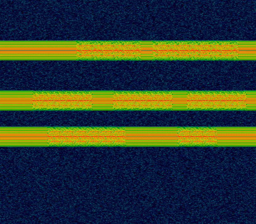
(Time is on the horizontal axis, frequency on the vertical – a bit different than a typical waterfall.) We can see there are three frequency bands in use here. It looks like each one starts and ends on idle, with occasional transmissions of some sort. We know we’ll need to tune to the center one. Let’s try doing this in GNU Radio.
GNU Radio
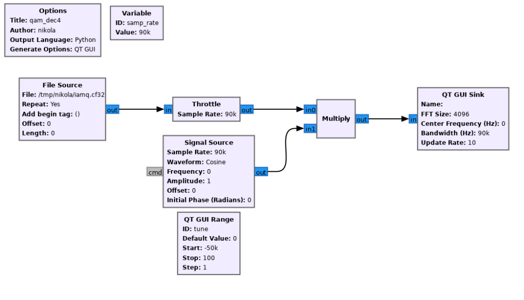
GNU Radio is a flow graph based software. Data flows from one block to the other. Let’s set up a simple graph to read in our file, at a given sample rate (I chose 90k arbitrarily) and visualize the data:
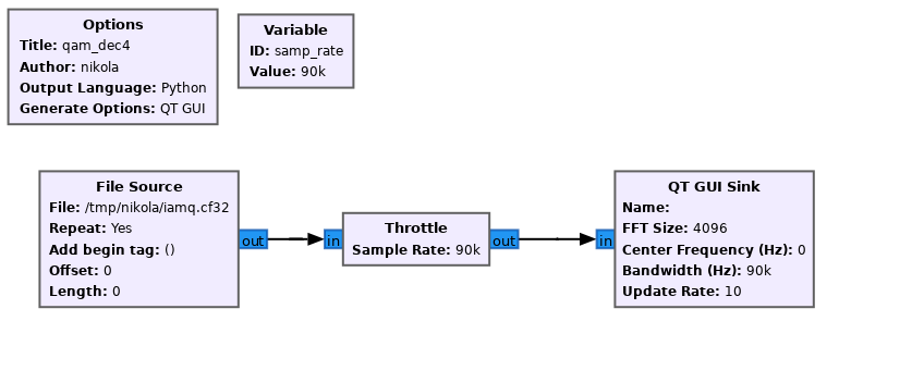
(The Throttle block is necessary so we don’t zoom through the entire file at CPU speed, but rather at a more natural transmission speed.) Note that if you set the File Source to Repeat, it will loop repeatedly. This can be useful so you don’t have to keep restarting the program.
Let’s run it:
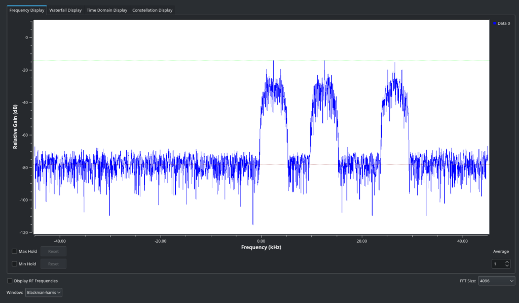
Yup, that’s our IQ file! But we’ll never be able to make sense of it when there’s multiple transmissions present. We need to tune to the right frequency, and then use a low-pass filter to filter out the transmissions that aren’t relevant (leaving just the middle one, as the challenge specifies).
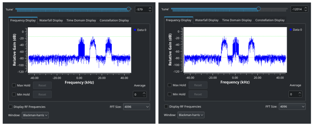
We can tune (frequency offset) by multiplying with a cosine, whose frequency we’ll control via a range slider:

We can move the slider until our middle transmission is roughly centered at 0 Hz:
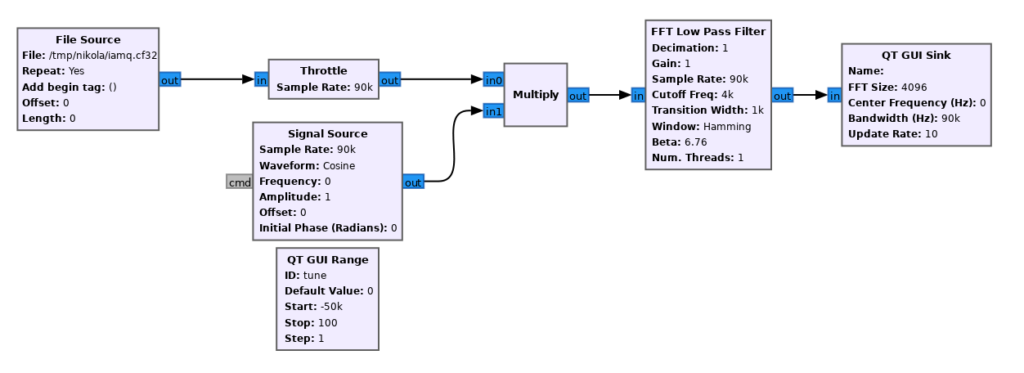
Now let’s use a low-pass filter to remove the other signals, leaving just ours. Note that the values here are arbitrary and will depend on your sample rate setting.
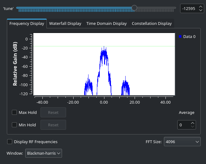
Note that we haven’t gotten rid of the other signals entirely, but remember the y-axis is logarithmic, so they have actually been considerably weakened. This will do.
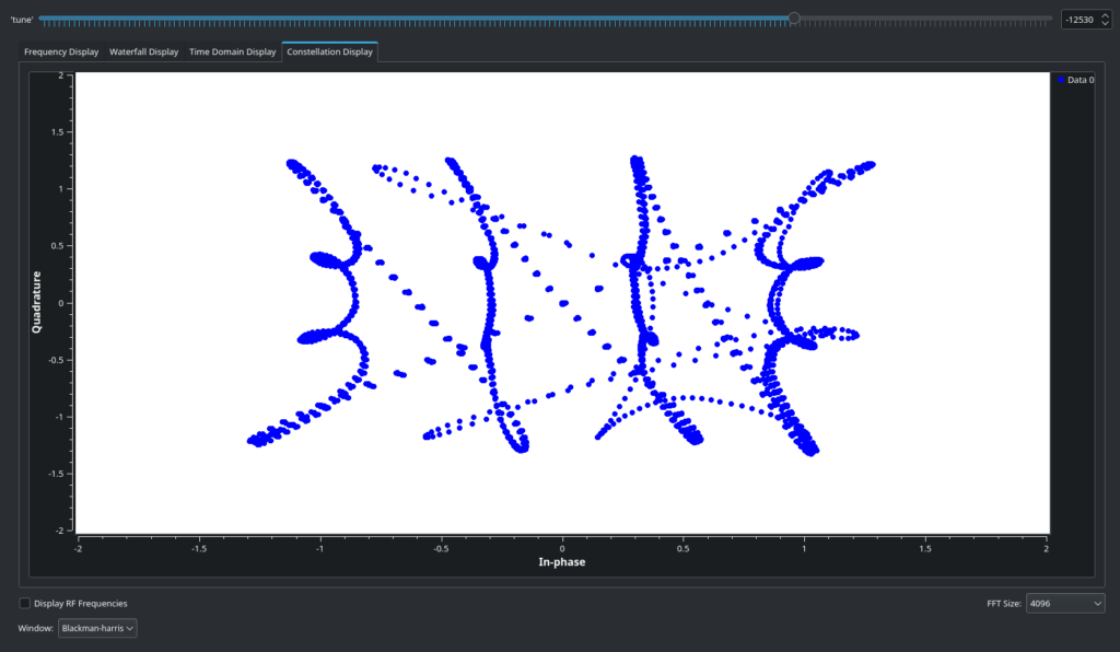
Our frequency shift isn’t quite right. We can tell because even if we get it close, if we go to the Constellation Display tab:

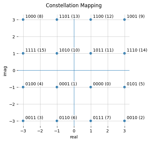
That is not a QAM16 constellation. Other sources can explain better what QAM is, but effectively, it’s a type of modulation where the amplitude and phase of the signal, together, represent a symbol in the data stream. The constellation display shows us the amplitude and phase of every sample of our signal on an X-Y scatter plot. A locked-in QAM signal should move around between a grid of points on this plane, as the image in the description showed:
If we get the frequency close but not quite, we can see the constellation almost looking as it should, but revolving in circles rapidly. We need to get the frequency finely adjusted.
Since this is a simulated signal, we actually could fiddle with it until the constellation stops spinning, but that won’t quite help us, since we also need to get the phase right – to make the constellation “stop spinning” in the proper, X-Y aligned orientation.
A DSP course would at this point probably get into PLLs or the Costas Loop or something. Unfortunately, I’m not an EE, and I can’t do any math beyond basic addition. Thankfully, GNU Radio allows me to be stupid: there’s a magic block for our purposes.
It’s called – you guessed it – Constellation Receiver:
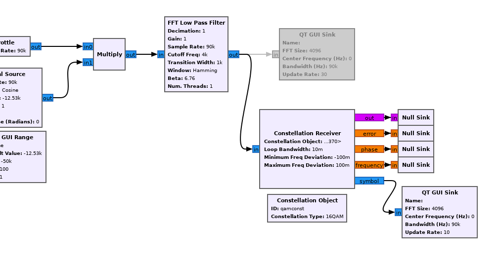
We need to provide it with a Constellation Object, which is in this case the default QAM-16. We also need to supply a bunch of parameters – truth be told, I just fiddled with them till they worked.
Let’s (D)isable the previous visualization, and examine the results of the Constellation Receiver.
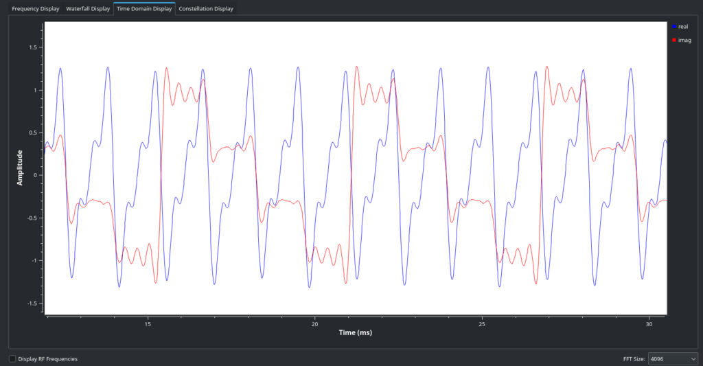
It’s hard to tell, but this is much better! You might notice it’s sweeping out the preamble/idle pattern mentioned in the description – going column by column, row by row. (This is if you happen to catch it during the preamble and not during a data transmission, which will look more chaotic but still clearly QAM-shaped). The Time Domain view will also show a QAM-16 signal:
Conveniently, this Receiver block will also attempt to extract QAM symbols by matching to the closest point in the constellation and decoding to the relevant 4-bit code. But we will need to do some downsampling – each symbol takes up multiple samples, and we want just one sample to be output per each symbol.
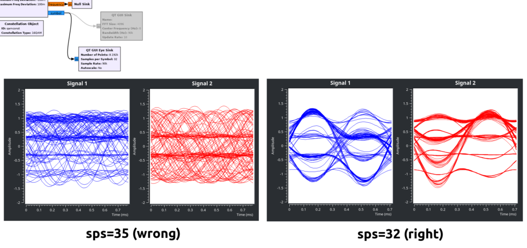
We can do some measurement on the time-domain view (changing the viz settings helps) to convince ourselves that in this capture, there are 32 samples per each data symbol. You can also figure out the value by bringing in an Eye Diagram and adjusting its samples-per-symbol parameter until you get a good looking eye pattern:
Getting Sloppy
An astute reader will notice that we never actually fixed the orientation of the QAM-16 square, beyond making sure it’s a square – we don’t know if it’s upside down, rotated 90 degrees, etc. A proper decoder would use the preamble/idle sequence to figure this out. It would also properly sample each symbol at its center. It would also probably use a matched RRC filter. And so on, and so forth.
We are playing a CTF. We won’t bother with all that.
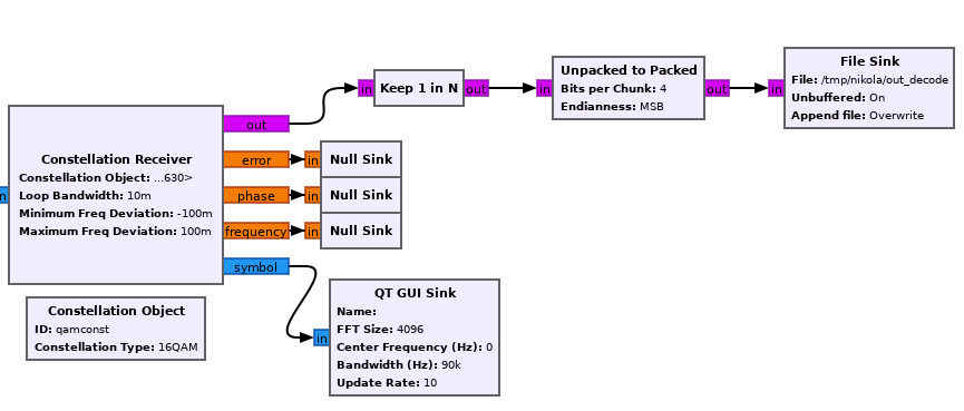
From the Constellation Receiver, we’ll tell GNU Radio to keep 1 in every 32 samples, pack two of them together (merging the nibbles into a byte), and then write the output to a file.
If you watch the constellation diagram, you’ll see that it rotates around periodically, the phase changing as the input file is looped. One out of every 4 times, it will be aligned properly. With our sample rate at 90k, this is enough – we can more or less brute force a proper alignment. Let’s run this and tail -f the output file.
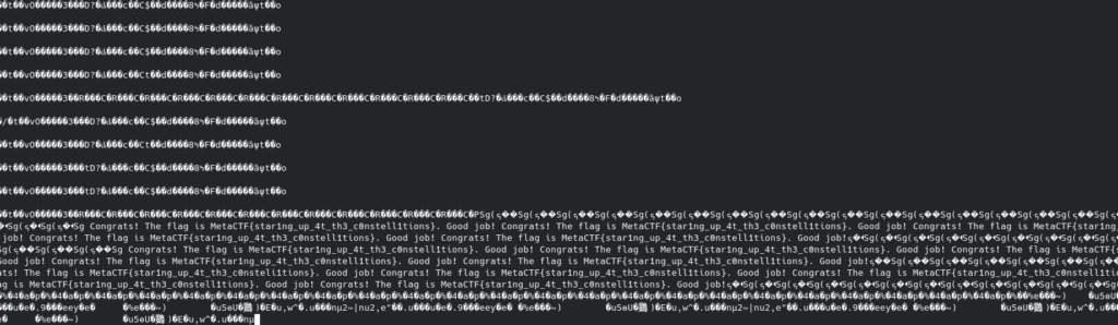
The reception isn’t great, but we can let it run a few times and manually fix up the flag, and there it is:
MetaCTF{star1ng_up_4t_th3_c0nstellations}
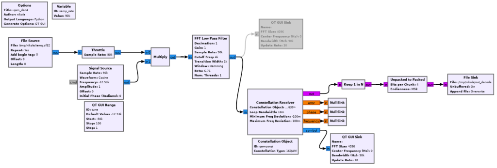
And here’s our final flow graph: